

| << Chapter < Page | Chapter >> Page > |
Because of the way computers are organized, signal must be represented by a finite number of bytes. This restrictionmeans that both the time axis and the amplitude axis must be quantized : They must each be a multiple of the integers. We assume that we do not use floating-point A/D converters. Quite surprisingly, the Sampling Theorem allows us to quantizethe time axis without error for some signals. The signals that can be sampled without introducingerror are interesting, and as described in the next section, we can make a signal "samplable" by filtering. In contrast,no one has found a way of performing the amplitude quantization step without introducing an unrecoverable error.Thus, a signal's value can no longer be any real number. Signals processed by digital computers must be discrete-valued : their values must be proportional to the integers. Consequently, analog-to-digital conversion introduces error .
Digital transmission of information and digital signal processing all require signals to first be "acquired" by acomputer. One of the most amazing and useful results in electrical engineering is that signals can be converted from afunction of time into a sequence of numbers without error : We can convert the numbers back into the signal with (theoretically) no error. Harold Nyquist, a Bell Laboratories engineer, first derived this result, known as the Sampling Theorem, in the1920s. It found no real application back then. Claude Shannon , also at Bell Laboratories, revived the result once computerswere made public after World War II.
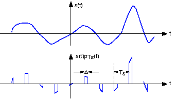
The sampled version of the analog signal
is
,
with
known as the
sampling interval . Clearly, the
value of the original signal at the sampling times ispreserved; the issue is how the signal values
between the samples can be
reconstructed since they are lost in the samplingprocess. To characterize sampling, we approximate it as
the product
,
with
being the periodic pulse signal. The resulting signal, as
shown in
[link] , has nonzero
values only during the time intervals
,
.
Sampled signal
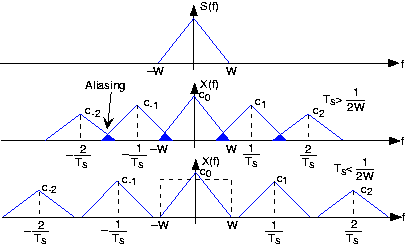
To understand how signal values between the samples can be "filled" in, we need to calculate the sampled signal'sspectrum. Using the Fourier series representation of the periodic sampling signal,
The Sampling Theorem (as stated) does not mention the pulse width . What is the effect of this parameter on our ability torecover a signal from its samples (assuming the Sampling Theorem's two conditions are met)?
The only effect of pulse duration is to unequally weight the spectral repetitions. Because we are only concernedwith the repetition centered about the origin, the pulse duration has no significant effect on recovering a signalfrom its samples.
The frequency , known today as the Nyquist frequency and the Shannon sampling frequency , corresponds to the highest frequency at which a signal can contain energy andremain compatible with the Sampling Theorem. High-quality sampling systems ensure that no aliasing occurs byunceremoniously lowpass filtering the signal (cutoff frequency being slightly lower than the Nyquist frequency) beforesampling. Such systems therefore vary the anti-aliasing filter's cutoff frequency as the sampling rate varies. Because such quality featurescost money, many sound cards do not have anti-aliasing filters or, for that matter, post-samplingfilters. They sample at high frequencies, 44.1 kHz for example, and hope the signal contains no frequencies above theNyquist frequency (22.05 kHz in our example). If, however, the signal contains frequencies beyond the sound card's Nyquistfrequency, the resulting aliasing can be impossible to remove.
To gain a better appreciation of aliasing, sketch the spectrum of a sampled square wave. For simplicityconsider only the spectral repetitions centered at , , . Let the sampling interval be 1; consider two values for the square wave's period:3.5 and 4. Note in particular where the spectral lines go as the period decreases; some will move to the left andsome to the right. What property characterizes the ones going the same direction?
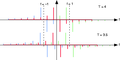
The square wave's spectrum is shown by the bolder set of lines centered about the origin. The dashed linescorrespond to the frequencies about which the spectral repetitions (due to sampling with ) occur. As the square wave's period decreases, the negativefrequency lines move to the left and the positive frequency ones to the right.
If we satisfy the Sampling Theorem's conditions, the signalwill change only slightly during each pulse. As we narrow the pulse, making smaller and smaller, the nonzero values of the signal will simply be , the signal's samples . If indeed the Nyquist frequency equals the signal's highest frequency, at least twosamples will occur within the period of the signal's highest frequency sinusoid. In these ways, the sampling signalcaptures the sampled signal's temporal variations in a way that leaves all the original signal's structure intact.
What is the simplest bandlimited signal? Using this signal, convince yourself that less than twosamples/period will not suffice to specify it. If the sampling rate is not high enough, what signal would your resulting undersampled signal become?
The simplest bandlimited signal is the sine wave. At theNyquist frequency, exactly two samples/period would occur. Reducing the sampling rate would result in fewersamples/period, and these samples would appear to have arisen from a lower frequency sinusoid.
Notification Switch
Would you like to follow the 'Analog-to-digital conversion' conversation and receive update notifications?

|
|

|
|

|
|

|
|

|
|
|
|
|

|
|

|
|

|
|

|