16.2 Entropy  (Page 2/8)

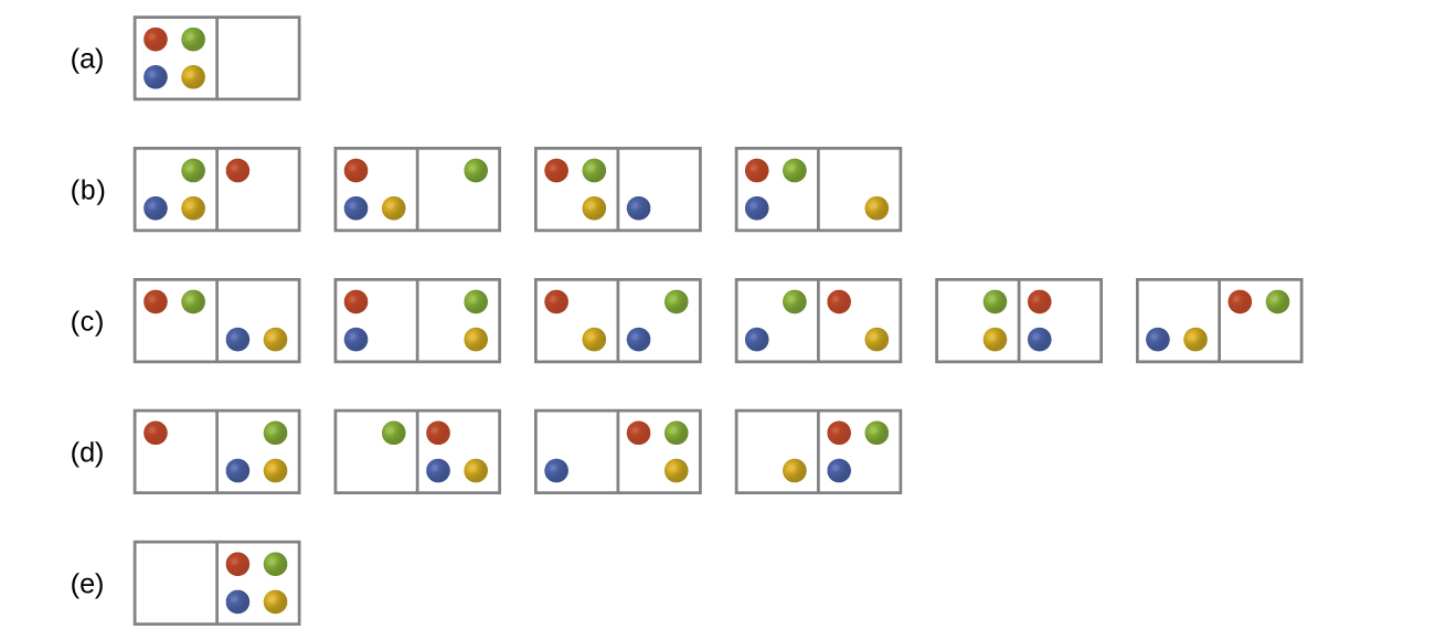
For this system, the most probable configuration is one of the six microstates associated with distribution (c) where the particles are evenly distributed between the boxes, that is, a configuration of two particles in each box. The probability of finding the system in this configuration is or $\frac{6}{16}$ or $\frac{3}{8}.$ The least probable configuration of the system is one in which all four particles are in one box, corresponding to distributions (a) and (d), each with a probability of $\frac{1}{16}.$ The probability of finding all particles in only one box (either the left box or right box) is then $\left(\frac{1}{16}+\frac{1}{16}\right)=\frac{2}{16}$ or $\frac{1}{8}.$

As you add more particles to the system, the number of possible microstates increases exponentially (2 ^N ). A macroscopic (laboratory-sized) system would typically consist of moles of particles ( N ~ 10 ²³ ), and the corresponding number of microstates would be staggeringly huge. Regardless of the number of particles in the system, however, the distributions in which roughly equal numbers of particles are found in each box are always the most probable configurations.

The previous description of an ideal gas expanding into a vacuum ( [link] ) is a macroscopic example of this particle-in-a-box model. For this system, the most probable distribution is confirmed to be the one in which the matter is most uniformly dispersed or distributed between the two flasks. The spontaneous process whereby the gas contained initially in one flask expands to fill both flasks equally therefore yields an increase in entropy for the system.

A similar approach may be used to describe the spontaneous flow of heat. Consider a system consisting of two objects, each containing two particles, and two units of energy (represented as “*”) in [link] . The hot object is comprised of particles A and B and initially contains both energy units. The cold object is comprised of particles C and D , which initially has no energy units. Distribution (a) shows the three microstates possible for the initial state of the system, with both units of energy contained within the hot object. If one of the two energy units is transferred, the result is distribution (b) consisting of four microstates. If both energy units are transferred, the result is distribution (c) consisting of three microstates. And so, we may describe this system by a total of ten microstates. The probability that the heat does not flow when the two objects are brought into contact, that is, that the system remains in distribution (a), is $\frac{3}{10}.$ More likely is the flow of heat to yield one of the other two distribution, the combined probability being $\frac{7}{10}.$ The most likely result is the flow of heat to yield the uniform dispersal of energy represented by distribution (b), the probability of this configuration being $\frac{4}{10}.$ As for the previous example of matter dispersal, extrapolating this treatment to macroscopic collections of particles dramatically increases the probability of the uniform distribution relative to the other distributions. This supports the common observation that placing hot and cold objects in contact results in spontaneous heat flow that ultimately equalizes the objects’ temperatures. And, again, this spontaneous process is also characterized by an increase in system entropy.