

| << Chapter < Page | Chapter >> Page > |
Estimate the area between the x -axis and the graph of over the interval by using the three rectangles shown in [link] .
![A graph of the parabola f(x) – x^2 + 1 drawn on graph paper with all units shown. The rectangles completely contained under the function and above the x-axis in the interval [0,3] are shaded. This strategy sets the heights of the rectangles as the smaller of the two corners that could intersect with the function. As such, the rectangles are shorter than the height of the function.](/ocw/mirror/col11964/m53485/CNX_Calc_Figure_02_01_008.jpg)
The areas of the three rectangles are 1 unit 2 , 2 unit 2 , and 5 unit 2 . Using these rectangles, our area estimate is 8 unit 2 .
Estimate the area between the x -axis and the graph of over the interval by using the three rectangles shown here:
![A graph of the same parabola f(x) = x^2 + 1, but with a different shading strategy over the interval [0,3]. This time, the shaded rectangles are given the height of the taller corner that could intersect with the function. As such, the rectangles go higher than the height of the function.](/ocw/mirror/col11964/m53485/CNX_Calc_Figure_02_01_009.jpg)
16 unit 2
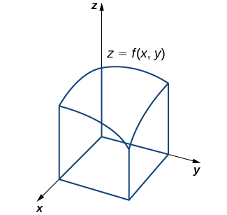
So far, we have studied functions of one variable only. Such functions can be represented visually using graphs in two dimensions; however, there is no good reason to restrict our investigation to two dimensions. Suppose, for example, that instead of determining the velocity of an object moving along a coordinate axis, we want to determine the velocity of a rock fired from a catapult at a given time, or of an airplane moving in three dimensions. We might want to graph real-value functions of two variables or determine volumes of solids of the type shown in [link] . These are only a few of the types of questions that can be asked and answered using multivariable calculus . Informally, multivariable calculus can be characterized as the study of the calculus of functions of two or more variables. However, before exploring these and other ideas, we must first lay a foundation for the study of calculus in one variable by exploring the concept of a limit.
For the following exercises, points and are on the graph of the function
[T] Complete the following table with the appropriate values: y -coordinate of Q , the point and the slope of the secant line passing through points P and Q . Round your answer to eight significant digits.
| x | y | m sec | |
|---|---|---|---|
| 1.1 | a. | e. | i. |
| 1.01 | b. | f. | j. |
| 1.001 | c. | g. | k. |
| 1.0001 | d. | h. | l. |
a. 2.2100000; b. 2.0201000; c. 2.0020010; d. 2.0002000; e. (1.1000000, 2.2100000); f. (1.0100000, 2.0201000); g. (1.0010000, 2.0020010); h. (1.0001000, 2.0002000); i. 2.1000000; j. 2.0100000; k. 2.0010000; l. 2.0001000
Notification Switch
Would you like to follow the 'Calculus volume 1' conversation and receive update notifications?

|
|

|
|

|
|

|
|

|
|

|
|

|
|

|
|

|
|

|