6.5 Physical applications

In this section, we examine some physical applications of integration. Let’s begin with a look at calculating mass from a density function. We then turn our attention to work, and close the section with a study of hydrostatic force.

Mass and density

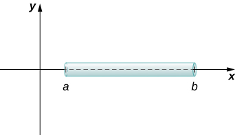
We can use integration to develop a formula for calculating mass based on a density function. First we consider a thin rod or wire. Orient the rod so it aligns with the $x\text{-axis,}$ with the left end of the rod at $x=a$ and the right end of the rod at $x=b$ ( [link] ). Note that although we depict the rod with some thickness in the figures, for mathematical purposes we assume the rod is thin enough to be treated as a one-dimensional object.

If the rod has constant density $\rho ,$ given in terms of mass per unit length, then the mass of the rod is just the product of the density and the length of the rod: $\left(b-a\right)\rho .$ If the density of the rod is not constant, however, the problem becomes a little more challenging. When the density of the rod varies from point to point, we use a linear density function    , $\rho (x),$ to denote the density of the rod at any point, $x.$ Let $\rho (x)$ be an integrable linear density function. Now, for $i=0,1,2\text{,…},n$ let $P=\left\{x_i\right\}$ be a regular partition of the interval $\left[a,b\right],$ and for $i=1,2\text{,…},n$ choose an arbitrary point $x_i^{*}\in \left[x_{i-1},x_i\right].$ [link] shows a representative segment of the rod.

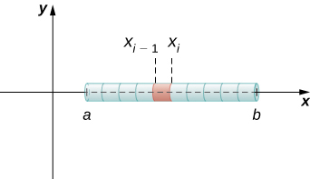
The mass $m_i$ of the segment of the rod from $x_{i-1}$ to $x_i$ is approximated by

Adding the masses of all the segments gives us an approximation for the mass of the entire rod:

This is a Riemann sum. Taking the limit as $n\to \infty ,$ we get an expression for the exact mass of the rod:

We state this result in the following theorem.

We apply this theorem in the next example.

We now extend this concept to find the mass of a two-dimensional disk of radius $r.$ As with the rod we looked at in the one-dimensional case, here we assume the disk is thin enough that, for mathematical purposes, we can treat it as a two-dimensional object. We assume the density is given in terms of mass per unit area (called area density ), and further assume the density varies only along the disk’s radius (called radial density ). We orient the disk in the $xy\text{-plane,}$ with the center at the origin. Then, the density of the disk can be treated as a function of $x,$ denoted $\rho (x).$ We assume $\rho (x)$ is integrable. Because density is a function of $x,$ we partition the interval from $\left[0,r\right]$ along the $x\text{-axis}.$ For $i=0,1,2\text{,…},n,$ let $P=\left\{x_i\right\}$ be a regular partition of the interval $\left[0,r\right],$ and for $i=1,2\text{,…},n,$ choose an arbitrary point $x_i^{*}\in \left[x_{i-1},x_i\right].$ Now, use the partition to break up the disk into thin (two-dimensional) washers. A disk and a representative washer are depicted in the following figure.